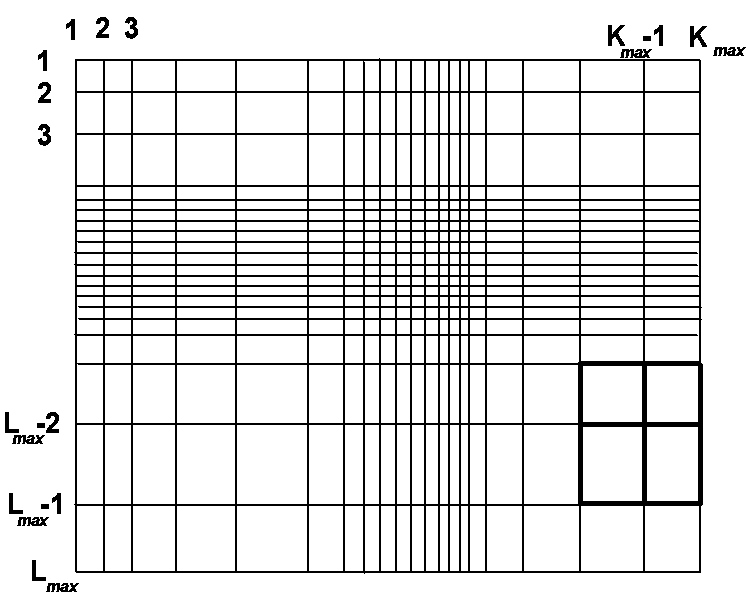
- We want to study models including important low velocity blocks, or layers, that occupy a relatively small parts of the grid. Then, with a spatially constant grid step size dictated just by the low-velocity regions (i.e. with regular fine grids) most parts of the models become oversampled.
- Using the heterogeneous formulation of the equations of motion, i.e. describing interfaces without explicit treatment of the traction-continuity condition, the resulting approximation at the interfaces is of a lower accuracy order (o(h), h being the grid step) as compared to the grid points outside the interfaces (o(h2)).
- Using the heterogeneous formulation up to the free surface, i.e. the so-called vacuum formalism (for more details see below) the free surface, in contrast to internal discontinuities, gets a stair-case ('zig-zag') form.
To be more specific, we concentrate on the spatial irregularity
hereafter called 'rectangular grids', the example of which is shown in
figure 1. Simply
speaking, any internal grid point has all eight necessary neighbouring
grid points: four on the central cross of the grid stencil, and the
complementary four points forming all together a rectangle. The
availability of all neighbours like this considerably simplifies
programming, while it still allows a great spatial variability of the
grid density. For similar grids and SH waves, see Moczo (1989), while
for a more general irregularity of the grid and SH waves, see Moczo et
al. (in press). For staggered irregular grids and P-SV waves, see
Jastram and Tessmer (1994); Falk et al. (1995).
Figure 1: An example of the irregular grid with a single grid stencil highlighted.
In this section we discuss which type of scheme is useful for the irregular grids. It is obvious that with a grid stencil containing simultaneously a small and a large grid 'leg', the scheme should be sensitive enough with respect to the exact position of an interface passing generally between the grid points. Most suitable schemes for this purpose are the so-called heterogeneous schemes.
Although the heterogeneous schemes have a long tradition in seismology, dating more that twenty years back to Boore (1972) and Kelly et al. (1976), they have been only recently theoretically justified. By justification we mean the proof that considering the equation of motion without the traction continuity condition, the latter can be automatically satisfied (approximated) by considering the material parameters as discontinuous functions (Zahradnik and Priolo, 1995). As a special case, the free surface may be approximated similarly to the internal grid point, while considering a part of its neighbourhood as the vacuum (Zahradnik et al., 1993; 1994b). However, as shown in Zahradnik (1995a) although the heterogeneous formulation of a differential equation can approximate the traction continuity, and the vanishing traction conditions, this property is not necessarily guaranteed for an arbitrary difference approximation to the differential equation of motion. Some FD schemes do approximate these conditions, while the others violate it. For example, the so-called short and full-form formulas for the mixed spatial derivatives can be used for internal grid points, but only the full-form scheme approximates properly the free surface. Of course, inside the medium the short form is preferable, because it is more economical.
Both short and full forms of the spatial mixed derivatives, as well as the standard forms for the non-mixed derivatives, should contain the geometrically averaged material parameters along the grid legs. Such an increase in complexity as compared to the schemes with local material parameters has practically no effect on the computing time, since the geometrical averages are evaluated only once, and stored in the operation memory; so the time needed to get them is a very small fraction of the entire FD run, as a rule. The need in the geometrically averaged parameters is not 'cosmetic', but it comes from the fact that the geometrical averages well represent a true position of the interfaces, hence the schemes become more accurate as compared to those with local parameters, and are free of stair-case artifacts at the interfaces. This has been shown both theoretically and numerically in (Zahradnik, 1995a), and agrees with the conclusions of Nielsen (1994) and Graves (in press).

Figure2: Two quarter-spaces model with irregular grid. S = line source (vertical force), R = receivers.
This philosophy stimulated us to start with the existing heterogeneous second-order scheme for P-SV waves, PS2, featuring all the advantages listed above, but developed for the regular square grids only (Zahradnik and Priolo, 1995), and the scheme has been quite recently generalized for the irregular grid (pp. 11-26 and Figs. 3.2-3.5 of Oprsal, 1996). The irregular-grid scheme has been called PSi2. Similarly to PS2, an analogy of the full form of the mixed spatial derivatives is employed in vicinity of the free surface (planar or non-planar), while an analogy of the short form is used elsewhere.
Using the vacuum formalism at a non-planar free surface has an important consequence. In contrast to the internal material discontinuities, the free surface gets a stair-case form. It is due to the fact that any geometrical average along a leg whose part (whatever small part) is in the vacuum becomes automatically zero-valued. This is why the vacuum formalism at the non-planar free surfaces is efficient with irregular grids, that allow a necessary refinement of the grid step size close to the non-planar topographic features, while, at the same time, they may keep a relatively coarse steps at the flat parts of the free surface.
Let's mention that we empirically found it possible to approximate both planar and non-planar free surfaces by the so-called air formalism, too. It means that the grid point at the surface, or in its vicinity, is again treated analogously as in the vacuum formalism, but instead of the vacuum (with the zero-valued material parametres) we take quite formally a medium with the P- and S-wave velocities of 300 and 0.01 m/s, and density of 0.01 kg/m3. In a numerical experiment with a step-like free surface of a homogeneous halfspace we proved that this approach gives synthetics that only negligibly differ from those computed by the vacuum formalism. (Two completely different codes were used for that comparison.) A similar method has been used by Mueller (1985).

Figure 3: Comparison between the PSi2 and SPEM results for the model of figure 2, receiver R2, the vertical component. Horizontal axis in seconds.
This observation offers an elegant way how a non-planar free surface can be simply introduced into various existing FD codes, simply including air blocks above the true surface of the elastic medium, while keeping the standard rectangular form of the FD computational domain. At the same time, using air instead of vacuum, there is no danger in unexpected divisions by zero during the FD calculation.
Due to the small values of the material parametres the grid doesn't transmit any waves in the air, so we don't have to worry about the grid step size in the air blocks. The grid steps are fully determined by the elastic part of the model. Such an approach is, of course, less efficient than the special code of Oprsal (1996). Less efficiency of the air formalism is due to the fact that in the air-points the FD calculation is formally performed, because the computational region is not restricted to the elastic part of the model. Another reason for less efficiency is that with the air-formalism the FD code should use the full form of the mixed derivatives everywhere. It is because we a priori don't know the location of the free surface, and the free surface needs the full form.
A practical complication, common either to the vacuum and air formalisms, is that certain configurations of the free-surface with respect to the grid legs are prohibited. These can be avoided by a perturbation of the model parametres (i.e. modification of the surface form) performed automatically in the FD program. For more details, see pp. 31-32 of Oprsal (1996).
An important problem related to the stair-case free surfaces in our FD programs is what happens at the corner points. To clarify this issue, Oprsal (1996), pp. 26-28, has applied the so-called consistency analysis of Zahradnik et al. (1993). It is the analysis of consistency of the FD scheme with the equation of motion and/or the free surface condition, based on the Taylor expansion of the displacement values present in the scheme. An interesting result is that at the 90-degree corners the PSi2 scheme approximates the free-surface conditions of a horizontal and vertical free surface, with an equal weight. In other words, it is equivalent to a local approximation of the corner by a 45-degree sloping surface (over one grid step).
As an example of the application of the PSi2 program on an irregular grid we present one model from Oprsal (1996). It is a two quarter-spaces model, shown in figure 2 and table 1.
| aI | bI | rI | aII | bII | rII | fmax* |
| 2000 | 1155 | 1000 | 3000 | 1732 | 2000 | 22 |
| Dt | Dxmin | Dzmin | Dxmax | Dzmax | Nt | K | L |
| 0.0001 | 0.8 | 0.8 | 4.0 | 4.0 | 4000 | 512 | 350 |
The grid is densified close to the horizontal free surface and the vertical interface. The synthetic seismograms calculated by PSi2 method (vertical component) are compared in figure 3 to those by Spectral Element Method (SPEM) of Priolo et al. (1994). The vertical dashed line in figure 3 shows the time window free of the spurious effects of the grid edges. The agreement with SPEM is excellent. The comparison between SPEM and the PSi2 scheme on a relatively coarse regular grid (step of 4m) was also performed (as in Zahradnik and Priolo, 1995), but here, in figure 3, the agreement is better, particularly in the arrow-marked parts.
Another important result from this experiments (and equally well from the other experiments of Oprsal, 1996) is that the PSi2 schemes allows an abrupt change in the grid step size, without numerical artifacts.
Next example shows the application of the PSi2 method to a topography model. It is a ridge-like model (figures 4,5, and tables 2, 3) taken from Gaffet and Bouchon (1989).
The comparison of the solutions on a coarse and fine regular grids, vertical components (figure 6), shows how the fine grid reduces the effect of the stair-case surface approximation. The comparison between the fine regular-grid solution and irregular-grid solution (figure 7, table4) shows no difference in the synthetics.
However, using the irregular grid needs 90 percent less memory and 95 percent less computer time. In this case the grid irregularity was again abrupt in vertical direction (changing from 3.333 to 33.33 m at the vertical coordinate of -6.666 m, and at the horizontal coordinate of 1000 m). A smooth transition from the fine to the coarse grid provided negligible differences.
| aI | bI | rI | fmax* |
| 2000 | 1000 | 1000 | 5.4 |
| Dt | Dx | Dz | Nt | K | L |
| 0.008 | 33.33 | 33.33 | 500 | 150 | 150 |
Table 3: The meaning of the variables is
as in table 2
| aI | bI | rI | fmax* |
| 2000 | 1000 | 1000 | 5.4 |
| Dt | Dx | Dz | Nt | K | L |
| 0.0016 | 6.667 | 6.667 | 2500 | 750 | 660 |
Table 4: The meaning of the variables is: aI, bI
- P, S wave velocities (m/s); rI
-density (kg/m3); fmax* -the frequency
(Hz) at which the absolute value of the spectrum is 1% of the maximum
spectral value; Dt -time step (s); Dxmin, Dzmin,Dxmin, Dzmin
are the minimum and the maximum grid steps (m) appearing in the model; Nt
-number of time steps; K, L -number of vertical and horizontal lines in
the model
| aI | bI | rI | fmax* | Dt |
| 2000 | 1000 | 1000 | 5.4 | 0.0008 |
| Dxmin | Dzmin | Dxmax | Dzmax | Nt | K | L |
| 3.333 | 3.333 | 33.33 | 33.33 | 10000 | 290 | 195 |
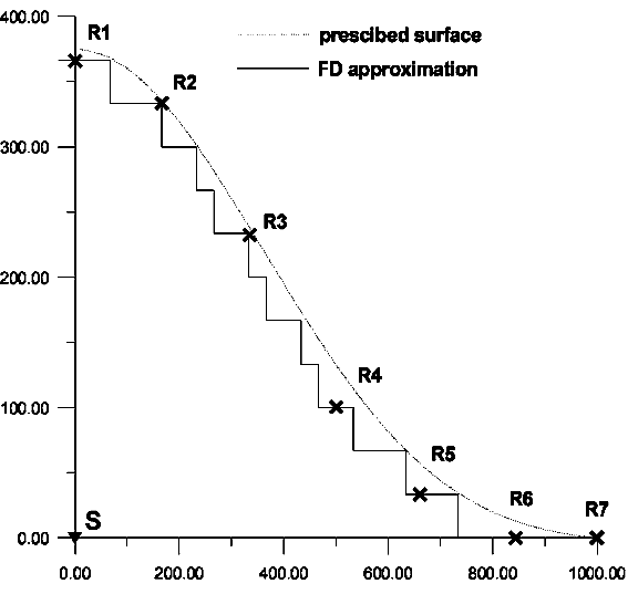
Figure 4: The ridge model M1 on a regular square coarse grid (the step of 33.33 m). S = source, R = receivers. All coordinates in metres.

Figure 5: The ridge model M2 on a regular square fine grid (the step of 6.67 m). S = source, R = eceivers. All coordinates in metres.

Figure 6: Comparison between the PSi2 results for models of figures 4, and 5 (the vertical component, the coarse and fine regular grids, M1 and M2; the seismograms on the coarser grid are undulated).

Figure 7: Seismograms (the vertical component) for the regular fine grid model M2, and the irregular grid model M3.

Figure 8: The sediment-filled valley model. The 16 blocks used in the FD modelling, and their material parameters, are shown. There are 49 equidistant receivers (not shown), distributed along the surface.
Hybrid methods are useful if a certain (smaller) part of the model is considerably more complex than the others. Let's call it 'localized inhomogeneity', which is embedded in a 'background' structure. The key point of the hybrid method is the representation of the complete wavefield by a sum of the 'background' and 'residual' parts. The background part can be calculated by a method cheaper than the FD method, e.g. by the DW method for 1D models, or the ray method for the 2D and 3D models. The residual part, that due to the localized 2D inhomogeneity, is assumed to require the FD method. The coupling between the background and the residual parts of the wavefield is based on the algorithm of Alterman and Karal (1968).
For the second-order FD schemes the coupling algorithm operates on two 'excitation lines', in our arrangement forming a rectangular 'excitation box' (two left and two right vertical lines, and two bottom horizontal lines). In our code the excitation box is attached to the free surface. This is because we are mainly interested in shallow subsurface structural complexities. The background field must be calculated for the entire time window of interest, before starting the hybrid calculation, and must be available along the lines of the excitation box. Then, inside the box, we numerically calculate (by FD) the complete wavefield, while outside the box, i.e. between the box and the 'non-reflecting' sides of the FD computational domain (Emerman and Stephen, 1983; Cerjan et al., 1985), the residual field is calculated by FD.

Figure 9: Synthetics (the horizontal component) for the surface receivers of the model shown in figure 8, excited by the SV plane wave vertically incident from below. Thick = hybrid A-FD method, thin = conventional excitation, i.e. with the plane wave excitation included during the FD modelling.
Very importantly, when introducing the localized inhomogeneity into the FD model, preparing for the hybrid coupling, the localized inhomogeneity must be fully contained inside the excitation box. In other words, the only changes between the background model and the hybrid model, present inside the FD domain, must be inside the excitation box. This is a crucial requirement of the hybrid method, dictating how the background and the residual structure and wavefield are defined. E.g., we cannot define the localized inhomogeneity as an additional surface layer, unlimited in a horizontal direction, if such a layer was missing in the background structure. At the same time, inside the FD domain, the medium surrounding the localized inhomogeneity during the hybrid calculation must have the same parametres as in the background field calculation. Deeper parts of the background model may be omitted, but it is already some approximation saying that the resulting solution doesn't contain any information about the interactions between the residual wavefield and the structural features deeper than the FD domain.
As an example we present a sediment-filled valley of figure 8. It is excited by a plane SV wave vertically incident from below. It is well known that excitation of the structures by plane waves in the FD models (operating on finite computational domains) is not easy. So-called non-reflecting conditions can be employed on the edges of the FD domain, but the left- and right-hand non-reflecting edges deform the excitation. Symmetry conditions at the left and right edges can be also used, with switching into non-reflecting edges after passage of the incident wave, but the switching can produce numerical problems in some models. Even worse deformation of the excitation takes place when the non-reflecting edges are combined with artificial tapers, or 'sponge layers' (Moczo, personal communication). Instead of these conventional approaches, here we show how the basin response to the plane-wave excitation of a short duration can be efficiently calculated by the hybrid method. It is an A-FD method. For the sedimentary valley of figure 8, the background structure is assumed to be represented by a homogeneous halfspace, and the background wavefield is simply a lagged sum of the incident SV wave and the wave reflected from the free surface. This sum is computed analytically at all grid points on the excitation lines, and stored on the excitation rectangle for all the grid points and time levels. Then, in the second step, the analytical solution is coupled with the FD method to produce the complete solution of the model including the basin. The considered spectral bandwidth is 0 to 13 Hz, while, with the grid step of 3 m, the accuracy is kept up to 5 Hz. The complete P-SV wavefield (horizontal component) is shown in figure 9, except the two traces on the top and bottom parts of the record section. The latter traces correspond to the residual wavefield.

Figure 10: The A-FD synthetics for the modified model of 8, i.e. the sediment-filled valley excluded. The top and bottom traces of zero residual field provide the methodical validation.
To check the accuracy of the method, the same is repeated for the background medium without the valley. As seen from figure 10, the method perfectly replicates the background wavefield inside the excitation box, while providing the zero-valued residual wavefield, as desired. It proves that the results of the hybrid calculation (figure 9) are free of numerical distortions caused by the propagation of the incident waves along the model edges, hence representing an improvement as compared to the conventional ('direct') FD calculations of the basin response due to the plane waves.
The next example involves a more realistic excitation of the same basin (that of figure 8), realized by an earthquake at the epicentral distance of 80 km. The effect of a point double-couple source, and the propagation in a horizontally layered crustal model is in this case calculated by the DW method (Bouchon, 1981; Kennett and Kerry, 1979). The source was located in the same vertical plane as that of the FD model. The details of the source and crustal model are unimportant for the present report (Caserta and Zahradnik, in preparation). The hybrid DW-FD calculation results are in figure12. The considered bandwidth and accuracy are the same as in figure 9.
It is to mention that in this example the (DW) excitation is no more prescribed just at the all employed grid points and time levels as in the preceding example, but in a series of equidistant points spaced by 15 m. The excitation was recorded with a time step 20-times larger than that of the FD method. Then, at each time level, the excitation has been linearly interpolated into the grid points. The interpolation is an important part of the algorithm, because (as a rule), the FD method requires a finer sampling than that necessary for the background wavefield. Another important issue is that the excitation lines spaced by a single grid step only are so close to each other that the same values can be used for each two neighbours. That means that the excitation should actually be computed for a single excitation line only (one left vertical, one right vertical, and one bottom horizontal), while copying the same values onto the neighbouring excitation lines. The latter simplification makes it possible to have the excitation completely independent of the employed FD grid. Then the same excitation can be used to re-run a given physical model on several different FD grids.
To examine the accuracy of the hybrid method, we now exclude the valley, and retain a homogeneous medium of the same parametres as the upper crustal layer. Now there is no reason to expect a completely vanishing residual field, because: (i) the background was a layered medium, while now we consider its upper layer only, and (ii) the excitation was due to a point source, hence with a 3D radiation pattern, while now we try to replicate it solely by a 2D (FD) method. Anyway, as seen from a very weak residual wavefield at the two top and bottom traces of figure 11, the coupling between the two methods performs well, hence the hybrid method provides encouraging results.
 Figure 11: Synthetics for the
modified model of figure 8, DW-FD method, an
earthquake excitation, i.e. with the sediment-filled valley excluded.
The two traces at the top and bottom, showing the zero-valued residual
wavefield, are validating the hybrid method.
Of course, with nearby sources, and/or the sources located off the FD plane, we expect much greater inconsistencies between the background 3D solution and the FD 2D solution. That's why our project assumes also an extension to the 2.5D FD method (Zahradnik, 1995b), the development of which has not yet been finished. So far, in cases marked by a significant 3D-2D inconsistencies, we simply pass from the DW-FD to the purely 2D hybrid FD-FD method (not presented here).
All the applications of the hybrid method presented above were for P-SV waves. It is to emphasize that P-SV in this context means the in-plane motion with respect to the FD plane, not with respect to the plane containing the source and the receiver. Using an arbitrary method to calculate the background field, we simply need to get 3 components, and to rotate them in- and out- of the FD plane. A new version of our hybrid code (under preparation) works simultaneously with P-SV and SH excitations. Getting FD response for both, we can use them to produce the transformation into any other coordinate system. We accentuate such a transformation because any combination of the P-SV and SH motions is more realistic as compared to the idealized pure P-SV or SH.
Attention should be always paid to the correct orientation of the displacement components. It is because the background and the complete wavefield are calculated by different programs, often with different orientation of the coordinate systems. For example, in the DW code the z-axis is positive upwards, while in the FD code the z-axis orientation is opposite. Errors in the component signs are not always quite obvious in the resulting synthetics. Sometimes the errors in the sign only yield a strong residual wavefield, hence they might be misinterpreted as inconsistencies between the 3D DW and the 2D FD solutions.

Figure 12: Synthetics (the horizontal component) for the model of 8, DW-FD method, an earthquake excitation. The two traces at the top and bottom display the residual wavefield. A slight 'ringing' in the middle right part of the figure is due to the high-frequency components inaccurately computed with the grid step of 3m.
For including absorption into the time-domain FD calculations, an accurate method of Emmerich and Korn (1987) is available. The E-K method, however, solves not only the partial differential equations of motion, but also an additional system of ordinary differential equations for auxiliary coefficients arising from the stress-strain relations, that significantly increase both the memory and computer time requirements of the method. An alternative approach is to calculate a 'perfectly elastic' impulse response of the medium (that of the non-absorbing medium), and to apply a subsequent absorption correction. Although the correction like that can handle an arbitrary frequency dependence of the quality factor Q(f), including various causal models, e.g. the Futterman model, it allows for a spatially invariable Q only. The method has been developed by Zahradnik et al. (1990a,b), independently of the analogous works of Vidale and Helmberger (1988). In spite of the strong assumption about the spatial constancy of Q, the method has been shown to provide a very good approximation to the exact method of the spatially dependent Q (Zahradnik et al., 1994a). The good agreement came from the fact that the mentioned applications concentrated on the models containing layers of very low velocities and Q's. In such models, the low velocity (low Q) layers dominate the absorption effect. Therefore a single-Q model, with Q chosen equal to that of the low velocity/low Q layer, did provide the good approximation. However, if our interest is in models with less contrasting velocities and Q's, and/or if we want to compare the synthetics on sediments and nearby rock outcrops, the space variability of Q becomes more important. This calls for approximate methods allowing for a spatially varying Q.
Among various Q(f) models there is a particular case of the linear
frequency dependence, Q=cf, enabling an easy consideration of the
spatial variability of Q during the time-domain simulations. As shown in
Zahradnik et al. (1990b), eqs. A12-A15, the linear Q model is equivalent
to including the first time derivative of the displacement into the
elastodynamic equation of motion. Assuming, for simplicity, Qp=Qs, and
denoting L1, L2 the spatial operators appearing in the 2D perfectly
elastic P-SV equations, the Q=cf model yields
|
|

- Many practical applications are restricted to relatively narrow frequency bands. In the narrow bands there is no much difference between different Q(f) models, provided the employed Q is taken with respect to the predominant frequency fp, and c=Q(fpr)/fpr.
The linear-Q model has been used to extend the existing PS2-based code (so far for a regular square grid only), and the following tests have been carried out :
1) It has been shown that the method gives the same results as those of the non-absorbing medium when a large Q is used, e.g. Q=1000 for shallow subsurface models.
2) It has been proven that with a spatially constant Q=cf the method gives the same impulse response as that obtained by the subsequent correction of the perfectly elastic response. In this particular case of the linear frequency dependence of Q the correction is a simple multiplication by an exponential time window exp(-p·(t-t)/c), t being semi-duration of the impulse.
3) The method has been found numerically stable in complex models with non-planar interfaces and several blocks with different Q's. An interesting observation was that in certain models calculated on a relatively coarse grids, where an unlimited growing high-frequency numerical ringing (instability) was present due to the numerical inaccuracy in the perfectly elastic case, the employment of the Q completely removed the ringing.
As an example let us present the sediment-filled valley of figure8, this time featuring Q = 5, 10, 20, and 50 in the blocks of Vs = 150, 300, 400 and 600 m/s, respectively. In this case the DW-FD method results in a considerably simpler response (figure 13) than that with no absorption (figure 12). Selected traces of figures 13 and 12 are compared in figure 14. Inside the valley the absorption effect is very well pronounced, while on the 'rock' outside the valley it becomes quite negligible.

Figure 14: Selected responses of the sediment-filled valley of figure 8 , DW-FD method. Thick = absorption considered, thin = absorption not considered.
It is to mention that quite recently a simple method for including a spatially varying Q into the FD calculation has been also proposed by Graves (in press). He is applying an exponential multiplication factor to the elastic wavefield at the end of each displacement update (time level). His method and our are formally different, but physically equivalent to each other.
An useful technical remark is that the method performs better with time functions whose spectra have zero or little energy at zero frequency. This result is based on a numerical experiment in which we compared the perfectly elastic responses with those calculated by our method with Q=1000. While the responses based on the time functions featuring the vanishing d.c. component provided an excellent agreement between the two approaches, the response based on a one-sided (delta-like) impulse performed not so well. We interpret this result as a failure at f=0, where our method implies a quite non-realistic value of Q=0, i.e. an infinitely large absorption.
The other program packages, so far developed only for regular square grids, include a simple spatially varying absorption model, and allow for hybrid coupling with independent methods. The performed tests with DW-FD method show that the source and path effects may be treated separately of the near-surface local effects, using a technique cheaper than FD, and coupled together with FD, where needed. The key point conditioning the successful coupling is the definition of the background and residual model features, and the two corresponding wavefield contributions. The tests provide the necessary experience with the technical details of the coupling that, very likely, will be useful for our long-term target project, i.e. the Ray-FD hybrid method.
The codes have been written in Fortran 77, as (mostly) machine independent. No parallelization, and no user-friendly interface have been included. The codes are available through Internet, upon request.
Boore, D.M. (1972). Finite-difference methods for seismic waves. In Methods in Computational Physics (B.A. Bolt, ed.), vol. 11, pp. 1-37, Academic Press, New York.
Bouchon, M. (1981). Simple method to calculate Green's functions for elastic layered media. Bull. Seism. Soc. Am. 71, 959-971.
Caserta A. and J. Zahradnik (1996). Modelling of strong ground motions combining deterministic and stochastic features - an application to the Tiber valley, Rome. Abstract. Europ. Seismol. Comm., Reykjavik.
Cerjan, C., D. Kosloff, R. Kosloff, and M. Reshef (1985). A non-reflecting boundary condition for discrete acoustic and elastic wave equations. Geophysics 50, 705-708.
Emerman, S.H. and R.A. Stephen (1983). Comment on Äbsorbing boundary conditions for acoustic and elastic wave equations", by R. Clayton and B. Engquist. Bull. Seism. Soc. Am. 73, 661-665.
Emmerich, H. and M. Korn (1987). Incorporation of attenuation into time-domain computations of seismic wave fields. Geophysics 52, 1252-1264.
Faeh, D., P. Suhadolc, St. Mueller, and G.F. Panza (1994). A hybrid method for the estimation of ground motion in sedimentary basins: Quantitative modeling for Mexico City. Bull. Seism. Soc. Am. 84, 383-399.
Falk, J., E. Tessmer, and D. Gajevski (1995). Tube wave modelling by the finite-difference method with varying grid spacing. EAEG meeting, Glasgow, talk D013.
Fukushima, Y., J.-Ch. Gariel, and R. Tanaka (1995). Site-dependent attenuation relations of seismic motion parameters at depth using borehole data. Bull. Seism. Soc. Am. 85, 1790-1804.
Gaffet, S. and M. Bouchon (1989). Effects of two-dimensional topographies using the discrete wavenumber - boundary integral equation method in P-SV cases. J. Acoust. Soc. Am. 85, 2227-2283.
Graves, R.W. (in press). Simulating seismic wave propagation in 3D elastic media using staggered-grid finite differences. Bull. Seism. Soc. Am.
Hestholm, S.O. and B.O. Ruud (1995). 2D finite difference elastic wave modelling including surface topography. Geophys. Prosp. 42,371-390.
Jastram, C. and E. Tessmer (1994). Elastic modelling on a grid with vertically varying spacing. Geophys. Prosp. 42, 357-370.
Kelly, K.R., R.W. Ward, S. Treitel, and R.M. Alford (1976). Synthetic seismograms: a finite-difference approach. Geophysics 41, 2-27.
Kennett, B.L.N. and N.J. Kerry (1979). Seismic waves in a stratified half space. Geophys. J. R. astr. Soc. 57, 557-583.
Moczo, P. (1989). Finite-difference technique for SH waves in 2-D media using irregular grids - application to the seismic response problem. Geophys. J. Int. 99, 321-329.
Moczo, P., P. Labak, J. Kristek, and F. Hron (in press). Amplification and differential motion due to an antiplane 2D resonance in the sediment valleys embedded in a layer over the halfspace. Bull. seism. Soc. Am.
Mueller, G. (1985). The reflectivity method: a tutorial. J. Geophys. 58, 153-174.
Nielsen, P. (1994). Numerical modelling of seismic waves: On the elimination of grid artifacts. Res. Rept., Norsk Hydro Res. Center.
Priolo, E., J. Carcione, and G. Seriani (1994). Numerical simulation of interface waves by high-order spectral modelling techniques. J. Acoust. Soc. Am. 95, 681-693.
Tessmer, E., D. Kosloff, and A. Behle (1992). Elastic wave propagation simulation in the presence of surface topography. Geophys. J. Int. 108, 621-632.
Vidale, J.E. and D.V. Helmberger (1988). Elastic finite-difference modeling of the 1971 San Fernando, California earthquake. Bull. Seism. Soc. Am. 78, 122-141.
Zahradnik, J., J. Jech, and P. Moczo (1990). Absorption correction for computations of a seismic ground response. Bull. Seism. Soc. Am. 80, 1382-1387.
Zahradnik, J., J. Jech, and P. Moczo (1990). Approximate absorption corrections for complete SH seismograms. Studia Geoph. et Geod. 34, 185-196.
Zahradnik, J., P. Moczo, and F. Hron (1993). Testing four elastic finite-difference schemes for behaviour at discontinuities. Bull. Seism. Soc. Am. 83, 107-129.
Zahradnik, J., P. Moczo, and F. Hron (1994). Blind prediction of the site effects at Ashigara Valley, Japan, and its comparison with reality. Nat. Hazards 10, 149-170.
Zahradnik, J., P. O'Leary, and J.S. Sochacki (1994). Finite-difference schemes for elastic waves based on the integration approach. Geophysics 59, 928-937.
Zahradnik, J (1995a). Simple elastic finite-difference scheme. Bull. Seism. Soc. Am. 85, 1879-1887.
Zahradnik, J. (1995b). Comment on Ä hybrid method for the estimation of ground motion in sedimentary basins: Quantitative modeling for Mexico City" by D. Faeh, P. Suhadolc, St. Mueller, and G.F. Panza. Bull. Seism. Soc. Am. 85, 1268-1270.
Zahradnik, J. and E. Priolo (1995). Heterogeneous formulations of elastodynamic equations and finite-difference schemes. Geophys. J. Int. 120, 663-676.
Zahradnik, J. and P. Moczo (in press). Hybrid seismic modelling based on discrete-wavenumber and finite-difference methods. Pure and Appl. Geophys.
